Modelling a dynamic entity-based decision table in an RDBMS
Usually local government units have different tax schedules for different types of fees. Let’s take for example taxes for businesses which is computed during renewal of business permits.
Table 1. Business Tax Schedule, with 2 Parameters
| Business Categories | Gross Sales | Tax |
|---|---|---|
| A | < 10000 | 198.00 |
| A | >= 10000 & < 15000 | 264.00 |
| A | >= 15000 & < 20000 | 362.00 |
| … | … | … |
| B | < 1000 | 21.60 |
| B | >= 1000 & < 2000 | 39.60 |
| B | >= 2000 & < 3000 | 60.00 |
| … | … | … |
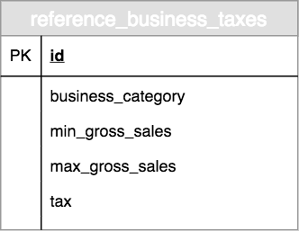
Given the table above, to determine the tax we need to know the Business Category and Gross Sales of the business. With that in mind we can think of representing this just a simple table, say reference_business_tax, with 4 fields : business_category , min_gross_sales, max_gross_sales, tax.
Image 1. UML ERD for table reference_business_tax
Hoping that tax schedules are that simple, then you encounter something like this within the same tax schedule:
Table 2. Continuation of Business Tax Schedule, with 3 Parameters
| Business Categories | Business Sub-Categories | Gross Sales | Tax |
|---|---|---|---|
| C | A | < 10000 | 99.00 |
| C | A | >= 10000 & < 15000 | 132.00 |
| C | A | >= 15000 & < 20000 | 181.00 |
| … | … | … | … |
| C | B | < 1000 | 10.80 |
| C | B | >= 1000 & < 2000 | 19.80 |
| C | B | >= 2000 & < 3000 | 30.00 |
| … | … | … | … |
Now with an additional parameter, Business Sub-Category, our original design doesn’t fit the tax schedule anymore. There are also other miscellaneous fees included in the computation that has their own reference fee schedule, like the fee for the Business Metal Plate:
Table 3. Metal Plate Fee Schedule
| Enterprise Scale | Metal Plate Fee |
|---|---|
| Micro-Industries | 200.00 |
| Cottage Industries | 200.00 |
| Small scale industries | 300.00 |
| Medium scale Industries | 1000.00 |
| Large scale Industries | 1000.00 |
The Metal Plate Fee uses a different set of parameters. If we are to model it, our original design can’t accommodate it and we have to create a separate reference table for it.
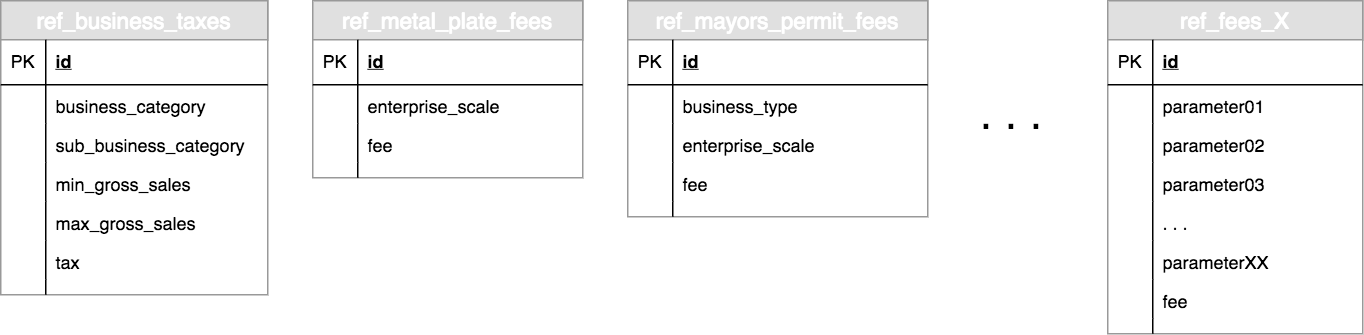
The challenge for a system like this is you can’t have just a single reference table that could accommodate all fee schedules, also you have to keep in mind that we are designing for the long-term use and maintainability of the product. If we are to create a reference table for each of the fees, then everytime there’s a change in the rules for deriving a business tax (ie. use a different parameter instead of Business Category, or add an additional parameter like Establishment Type) then it would require us to remigrate the tables, the same case would be if there are any other new fees that are introduced through ordinances (see sample reference tables in Image 2). That doesn’t make the system maintainable and could potentially explode to X number of tables.
Image 2. Sample reference tables
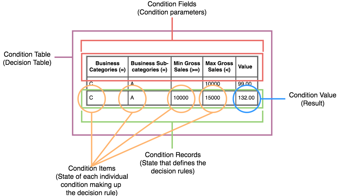
Instead of creating a reference table for every fee, we can make use instead of decision tables. A decision table contains decision rules which is composed of the conditions, the conditions states, and the desired actions or results for each state. The structure of a decision table may vary depending on the implementation. In our case we represent the decision table in this manner:
Image 3. Different components of a decision table
Modelling our solution:
Image 4. UML ERD for our decision table implementation
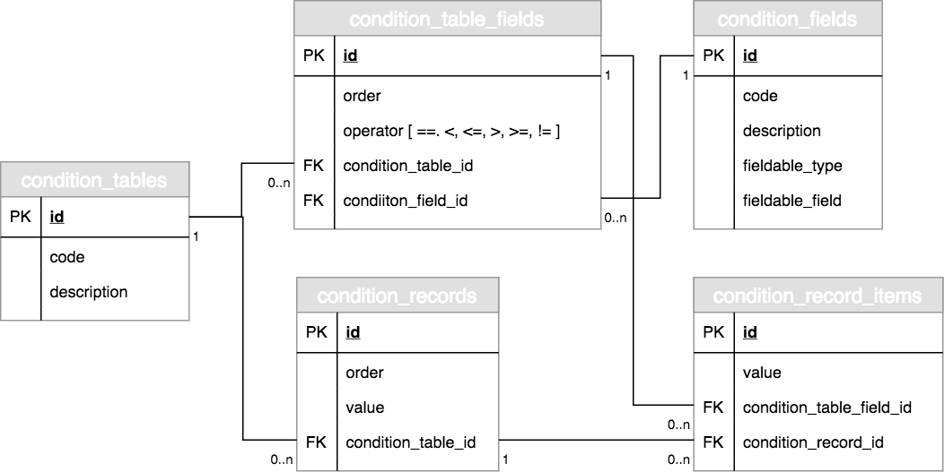
Following the design above would allow us to model any decision table based on any entity in the system.
Instead of creating database tables for different fees, we could just create records condition_tables table.
For the columns of the fee table, we create records in condition_fields table and associate it to condition_tables through condition_table_fields.
For every row in the fee table, we create records in condition_record.
For each cell in the row, just create a record in the condition_record_items table and associate it to the corresponding condition_record.
Let’s simulate how the table records would look like for Business Tax (with 3 parameters):
Image 5. Relationship of Condition Table and Condition Fields
In the diagram above we have a record in condition_tables table for CTBTX which represents the condition table for Business Tax.
Condition table CTBTX has the following columns: Business Categories, Minimum Gross Sales, and Maximum Gross Sales, which are defined by the following records in condition_fields table, respectively: CFBCT, CFNGR, and CFXGR.
You might ask, where do condition fields come from? Condition fields are just fields from any other table in the system. For example there may be a business_categories table with the field code, and business_earnings table with the field gross. This makes the creation of condition tables truly dynamic, allowing field from any table in the system to be part of the data structure definition.
The condition fields are associated to the condition table through the condition_table_fields table. Each record in the condition_table_fields table represents a column in the condition table it is associated to (A). The ordering of the columns from left-to-right for a specific condition table is denoted by the order field. All condition_table_fields records are also associated to the condition fields they represent (B). Using these associations we can model each column in the condition table (C). Also, take note of the oper field in condition_table_fields table, it will be useful later as we go through the individual rows in the condition table.
Image 6. Relationship of Condition Records to the Condition Table
The next component that makes up the structure of a condition table are its rows. Each row in the condition table represents the needed state of each parameter to be able to obtain the value at that row. For example, in Image 6, to get the value 264, the Business Category should be = ‘A’, Minimum Gross Sales should be >= 10,000.00, and Maximum Gross Sales should be < 15,000.00. Now if you notice, this is where the oper field comes in. The specific values per parameter should satisfy the conditional operator defined by oper.
Rows of the condition table are maintained in the condition_records table. Each record is associated to the condition table it belongs to (D), and each record represents one row in the condition table (E). The output value for a specific row is also stored in the condition_records table (F).
Image 7. Relationship of Condition Record Items to the Condition Record
The expected state for each parameter per row is stored in the condition_record_items table. Each record in condition_record items, represent a single cell for a specific row in the condition table it is associated to (G).
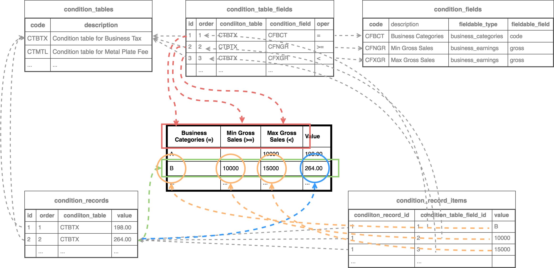
Here’s a mapping of the entire condition table data structure:
Image 8. Full mapping of the condition table data structure
Now that the condition table structure is complete, next is we have to be able to retrieve values from the condition table. The retrieval process is fairly simple. Assuming we have this JSON as input:
{
  "params" : {
    "condition_table" : "CTBTX",
    "inputs" : [
      { "condition_field" : "CFBCT", "value" : "B" },
      { "condition_field" : "CFNGR", "value" : "12000" },
      { "condition_field" : "CFXGR", "value" : "12000" }
    ]
  }
}
To be able to retrieve the corresponding condition table entry we just have to access the condition table indicated in the input param, then traverse each condition record of that condition table, then for each condition record traverse each condition record item comparing it to its corresponding input determined by the order of the condition field. Operator used for comparison is the one defined in the condition table fields entry. The input will only be considered as match if all comparison returns true. The condition record value for the first condition record that matches the input is returned and traversal immediately stops.
Image 9. Retrieval from a condition table